


MIGAL.CO Sensorbox – Capture, Understand, and Connect Welding Process Data
- Time-synchronized multi-sensor capability: Current, voltage, wire feed and gas flow with a common time base
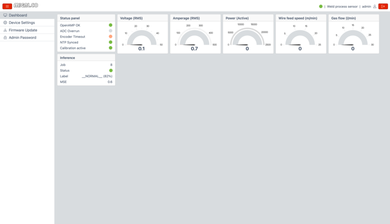
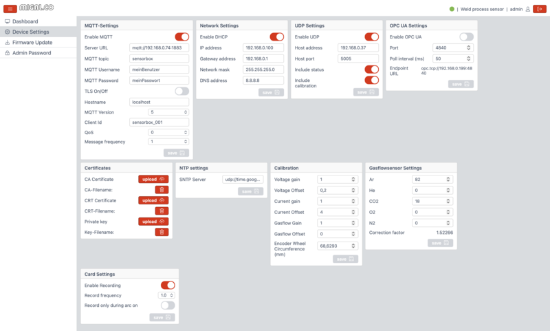
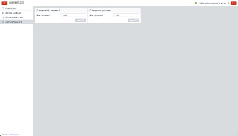
- Web dashboard for configuration, live display, and firmware updates
- 5 kHz sampling rate: According to the sampling theorem, frequency components up to approx. 2.5 kHz (Nyquist frequency) can be unambiguously measured
- High-speed raw data stream (UDP) for oscilloscope traces, FFT, U-I diagrams and histograms – ideal for test series and model development
- Deterministic measurement windows & sequence numbers (timestamp + seq) for reproducible evaluation and packet loss detection
- On-device feature calculation (U/I RMS, active power, statistical values) for rapid parameter determination without PC/cloud
- MQTT/JSON telemetry for easy integration into laboratory setups, data pipelines and time-series databases (e.g. InfluxDB)
- OPC UA Server – standardized interface for industrial integration
- Diagnostic and quality flags in the data stream (e.g. ADC overrun, encoder timeout, NTP sync) for clean data validation
- Dual-core architecture (measurement core + communication core) for stable measurement even under network and UI load
- NTP synchronization for comparable timestamps across multiple Sensorboxes/welding stations
- RoboScope (Windows/macOS) for live analysis: oscilloscope, FFT, waterfall diagram, histogram, U-I and U-I density – quickly from "signal" to "insight"
- Calibratable via zero point, gain, and encoder wheel circumference
- Integrated correction factor calculation for arbitrary gas mixtures of Ar, He, O₂, H₂ and N₂
- Export function of measurement data in the weldx format
- Direct transfer of measured values into WPS-Maker documents
- Storage and centralized monitoring in RoboCenter
- Modbus TCP (Port 502) - SPS-connection via Standard-Modbus-Protokol (Holding Registers)
- SD card logging (CSV) – automatic, NTP-synchronised recording of voltage, current, wire feed speed and shielding gas flow to microSD card, with configurable interval and daily file rollover
- AI-assisted anomaly detection and fault classification
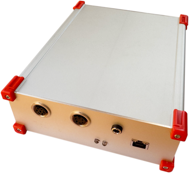
The MIGAL.CO Sensorbox is a modular, microcontroller-based measurement and communication platform for high-resolution acquisition, processing, and forwarding of welding process data for arc welding processes. It was developed for the harsh industrial welding environment and forms the technical foundation for process monitoring, data-based quality analysis, and prospectively AI-supported defect detection.
With the Sensorbox, the user obtains welding data directly from the process – cleanly time-stamped, structurally packetized, and securely transmitted to the network. This enables:
- Making welding processes transparent (instead of relying on "gut feeling")
- Tracing parameters per weld seam / job / workstation
- Feeding data into InfluxDB, dashboards or cloud systems
- Implementing real-time visualization (oscilloscope/spectrum) or edge analytics
- Establishing the foundation for automated anomaly and defect detection
- Quickly and easily creating Welding Procedure Specifications (WPS) from real, measured welding data
System Architecture: Real-Time Measurement Meets Network & Analysis
Inside, an STM32H7 dual-core (Cortex-M7 + Cortex-M4) operates with a clear division of tasks:
- Cortex-M4: handles the time-critical measurement (high-frequency, deterministic)
- Cortex-M7: takes care of data preparation, analysis, protocols, network communication, and system control
Both cores exchange data via OpenAMP / RPMsg – with low latency, clear sequencing, and a robust structure.
Measured Variables: The Most Important Process Parameters Captured Synchronously
The Sensorbox currently captures:
- Welding current
- Welding voltage
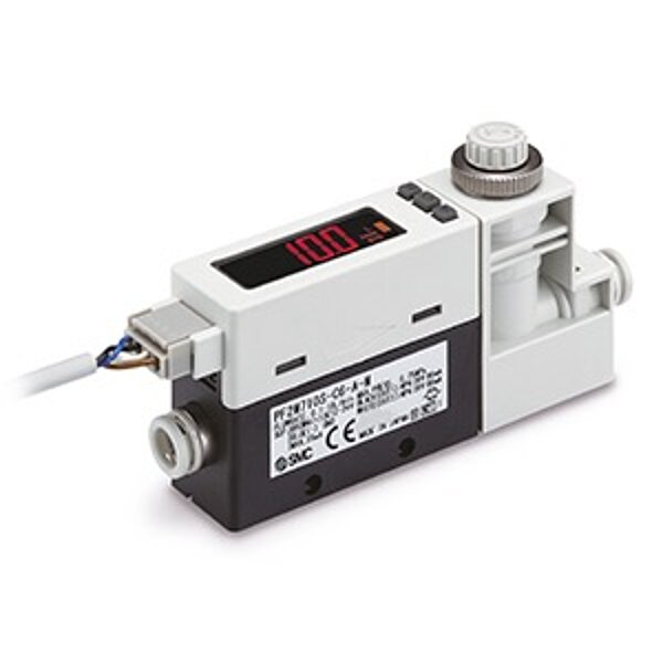
- Gas flow rate
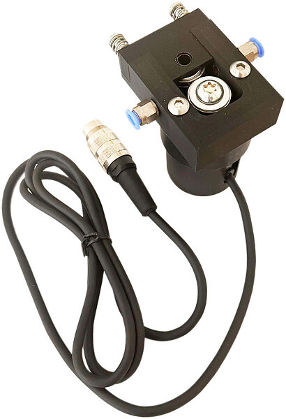
- Wire speed
Current & voltage are acquired with high temporal resolution via the STM32H7 ADCs in DMA circular mode. A 5 kHz sampling rate is achieved.
Gas flow rate and wire speed are fully integrated and are recorded synchronously with the electrical variables – ensuring time reference and correlation across all parameters.
Each measurement frame contains, in addition to the raw data, important metadata such as:
- Timestamp
- Sequence number
- Status flags
- Calibration parameters (gain/offset)
This allows raw data to be accurately converted into physical quantities on downstream systems – reproducibly and traceably.
Data Processing: Key Figures Calculated Directly on the Device
On the Cortex-M7, data is already preprocessed and analyzed. Currently available features include:
- RMS and mean value calculation
- Active power from current and voltage
- Scaling & acquisition of gas flow rate and wire speed
The data is then structured into packets and tagged with unique identifiers, so it can be clearly assigned to a job, a weld seam, or a workstation.
Communication & Networking: Securely into IT – Fast into Real-Time
The Sensorbox is fully network-capable via Ethernet (LwIP TCP/IP stack) and offers two central data paths:
MQTT over TLS (mbedTLS) – for IT, Cloud & Databases
Process data (current, voltage, gas, wire) is transmitted cyclically (typically 0.1 to 5 seconds) – ideal for:
- Cloud/server connections
- Process monitoring & reporting
- Storage in time-series systems (e.g. InfluxDB)
- Secure integration into existing IT infrastructure
UDP Real-Time Stream – for High-Frequency Live Data
For high-frequency and latency-critical applications, there is also a UDP data stream. Through this, raw measurement frames (current/voltage) can be sent to external systems with virtually no delay.
The UDP packets contain structured headers (including magic number, sequence numbers, timestamps, payload description) – ensuring that synchronization, validation, and traceability remain robust even in case of packet loss.
Typical use cases:
- Live visualization (oscilloscope or spectral display)
- Fast control/assistance systems
- Edge- or PC-based online analysis
Additionally, an integrated web server (Mongoose) is on board – for diagnostics, configuration, and future visualizations.
OPC UA Server – Standardized Interface for Industrial Integration
For easy connection to SCADA/MES/IIoT platforms, the Sensorbox provides an OPC UA server (opc.tcp). This allows welding data to be read out vendor-neutrally and without proprietary gateways by OPC UA clients such as UaExpert or Node-RED.
Provided measured values (read-only):
- Current (RMS) [A]
- Voltage (RMS) [V]
- Power [W]
- Gas flow [l/min]
- Wire speed [m/min]
The values are cyclically updated and are available in namespace ns=1 – ideal for live monitoring, data logging, or further processing in higher-level systems.
Time Base & Synchronization: Data with Absolute Time Reference
For precise temporal classification, the Sensorbox supports SNTP/NTP time synchronization. All measured values are tagged with absolute timestamps – important for:
- Correlation of multiple Sensorboxes
- Clean time-series analysis
- Later evaluation in InfluxDB & similar systems
Persistence & Configuration: Robustly Stored, Even During Power Drops
Device, network, and security parameters (e.g. IP configuration, MQTT credentials, UDP target address, TLS certificates) are persistently stored in internal flash.
A robust storage strategy with:
- Magic number
- Checksums
- Clearly defined flash sectors
ensures that configurations are preserved even during unexpected power loss.
SD Card Logging: Recording Process Data Locally and Network-Independently
Regardless of network availability or IT infrastructure, the Sensorbox can write process data directly to an inserted microSD card in CSV format — robust, straightforward, and immediately ready for analysis.
Each row contains an NTP-synchronised timestamp along with the current values for voltage, current, wire feed speed, and shielding gas flow. The data is directly usable in Excel, Python, or any analysis tool of your choice.
Configurable parameters (via web dashboard):
- Logging interval — freely selectable (e.g. 0.1 to 5 seconds)
- Arc filter — optionally log only during an active welding process
- Enable / disable — via dashboard
Files are organised by date (YYYY-MM-DD.csv) with automatic rollover at midnight. A sync to the card is performed after every write operation, ensuring that no data is lost even in the event of an unexpected power failure.
Typical use cases:
- Long-term recording over days or weeks
- Backup in addition to MQTT transmission
- Rapid commissioning — insert card, enable logging, done
- Optional standalone operation without a network (e.g. on a construction site or in the field) — requires a coin cell battery
In Brief
The MIGAL.CO Sensorbox is the bridge between the welding process and the data world:
Precise measurement, synchronized process data, on-device preprocessing, and secure or real-time-capable transmission – ready for monitoring, analysis, and the next level of quality assurance.
Messverfahren für Strom, Spannung und Leistung
Measurement Methods for Current, Voltage, and Power
The MIGAL.CO Sensorbox calculates precise process parameters for voltage, current, and power from high-frequency raw data at a 5 kHz sampling frequency. Voltage u(t) and current i(t) are captured in short time windows and digitally evaluated:
- RMS Voltage (U_RMS) and RMS Current (I_RMS) are the so-called effective values. They reliably describe the electrically "effective" quantity even when the signal is not sinusoidal – as is typical in welding.
- Power (P) is calculated as the mean of the instantaneous power: For each sample, u × i is computed and then averaged over the time window. This produces a stable power value that cleanly reflects real process changes (e.g. short-circuit phases, arc instability, wire/gas influences).
These key figures form the basis for live monitoring, trend analyses, quality evaluation, and subsequent AI-supported defect detection.
RMS-Voltage:
\[ U_{\mathrm{RMS}}=\sqrt{\frac{1}{N}\sum_{k=0}^{N-1} u[k]^2} \]
RMS-Current:
\[ I_{\mathrm{RMS}}=\sqrt{\frac{1}{N}\sum_{k=0}^{N-1} i[k]^2} \]
Mean Active Power:
\[ P=\frac{1}{N}\sum_{k=0}^{N-1}\big(u[k]\cdot i[k]\big) \]
Technical data
| Interface | Ethernet (10/100 Mbit/s) |
| Data transmission protocol | MQTT (3.1.1 and 5), UDP, OPC UA, Modbus TCP |
| Web interface | For configuration and real-time display |
| Supply voltage | 9 - 12 Volts DC |
| Network | DHCP, static IP |
| Message frequency | MQTT: 0.1 - 5 per second, UDP: ~20 frames × 256 values per second = 5 kHz |
| Encryption | MQTT: TLS 1.3, UDP binary unencrypted |
| Sensorbox dimensions | 200 x 160 x 60 mm (L×W×H) |
| Sensorbox weight | 1.1 kg |
| Protection rating | IP 20 |
| Voltage measurement | - 60 to + 60 Volts (AC, DC), +/- 1% of full scale |
| Current measurement | - 600 to + 600 Amperes (AC, DC), +/- 1% of full scale |
| Wire diameter range | 0.8 mm – 1.6 mm (larger on request) |
| Encoder resolution | 0.114 mm, 600 pulses per revolution |
| Wire feed speed | 0 - 20 m/min |
| Wire speed accuracy | 0.7% at 10 m/min and 0.1 s sampling interval |
| Encoder weight | 0.40 kg |
| Gas flow rate | 0.5 - 50 l/min |
| Gas flow accuracy | +/- 3% of maximum value |
| Gas flow sensor weight | 0.10 kg |


MQTT-Message
The Sensorbox transmits its measurement and status data in a compact JSON (JavaScript Object Notation) format. Each message corresponds to a temporally uniquely assignable snapshot of the welding process and contains both process key figures and system states and firmware versions.
Time & Sequence
→ Used for synchronization with other systems (InfluxDB, dashboard, RoboScope, MES).
→ Allows detection of dropouts, packet loss, or gaps in the recording.
Electrical Key Figures
→ These quantities enable load/energy analysis, process stability assessment, and comparison of jobs/parameters.
Wire & Gas
→ Basis for process monitoring (e.g. insufficient feed, wire jamming, defect detection).
→ Already corrected in the Sensorbox so that the user directly receives a practically relevant value.
→ Transparency on how much raw values have been adjusted due to calibration/environmental influence.
Status Object (Health & Diagnostics)
Under status, important diagnostic flags are provided as booleans:
→ This enables remote diagnostics without the user needing direct access to the hardware.
Firmware Versions (Traceability)
Example:
{
  "ts": "2026-01-21T10:15:23.123Z",
  "seq": 4711,
  "u_rms": 23.45,
  "i_rms": 156.78,
  "p_rms": 3680.2,
  "wire_m_min": 8.50,
  "gas_l_min": 12.30,
  "gas_cf": 1.07,
  "status": {
    "openamp_ok": true,
    "adc_overrun": false,
    "encoder_timeout": false,
    "ntp_synced": true
  },
  "fw": {
    "m7": "1.0.3",
    "m4": "1.0.3"
  }
}
UDP High-Speed Stream (Raw Data Packet)
For high-resolution analysis (oscilloscope view, histograms, event detection), the Sensorbox additionally sends a binary/CSV-like UDP data stream alongside the JSON telemetry. Each UDP packet contains a header with metadatafollowed by a block of ADC raw samples for voltage and current.
1) Packet Header (Metadata)
→ This allows the receiver to reliably identify data as a "Sensorbox frame" and discard erroneous or foreign packets.
Timestamp in milliseconds.
→ Enables time-correct display (e.g. live trace), logging, and synchronization with other sources.
Sequential sequence number.
→ Packet losses or ordering errors (UDP!) become immediately visible.
Number of samples per channel in this packet.
→ A packet is a "data block" (frame) with a precisely defined scope.
Current gas flow rate (l/min) as meta-information for the sample block.
→ Practical for directly correlating oscilloscope data with process parameters.
Wire feed speed (m/min) at the same point in time.
→ Can be 0 if the wire is stationary or an encoder/signal problem exists.
Bitmask for system states/error flags (e.g. ADC overrun, encoder timeout, OpenAMP OK, NTP sync).
→ Diagnostics without extra queries – each packet carries its health status.
Calibration/conversion parameters.
→ This allows the receiver to convert raw data to physical quantities (or deliberately store raw data and reconstruct later with the same parameters).
2) Sample Data (Payload)
After the header, a table/sequence follows:
→ From this, the receiver can:
- Generate oscilloscope traces (u(t), i(t))
- Calculate RMS/power/arc stability
- Detect peaks, short circuits, spatter events
- Create histograms/distributions (e.g. current distribution per job)
Why UDP?
UDP is ideal for live streaming large data volumes:
- Very low latency
- Low protocol overhead
- "Best effort" (packet loss possible) → therefore: seq in header
For robust storage/backfill, the "slow" telemetry channels (e.g. JSON via MQTT/HTTP) are usually used in parallel, while UDP serves for real-time viewing (RoboScope).
Example Python code for outputting the UDP stream in the terminal (call e.g. with python3 udp_dump.py 9000):
#!/usr/bin/env python3
import argparse
import socket
import struct
import math
MAGIC_OSCI = 0x3143534F  # "OSCI"
FLAG_STATUS = 0x0001
FLAG_CAL    = 0x0002
BASE_HDR_FMT = "<IHHII"              # magic, header_len, flags, seq, sample_cnt
BASE_HDR_LEN = struct.calcsize(BASE_HDR_FMT)  # 16
def parse_packet(buf: bytes):
    if len(buf) < BASE_HDR_LEN:
        return None
    magic, header_len, flags, seq, sample_cnt = struct.unpack_from(BASE_HDR_FMT, buf, 0)
    if magic != MAGIC_OSCI:
        return None
    # Minimaler Header: base + ts + meta
    if header_len < (BASE_HDR_LEN + 8 + 8) or header_len > len(buf):
        return None
    off = BASE_HDR_LEN
    ts_ms, = struct.unpack_from("<Q", buf, off)
    off += 8
    gas_l_min, wire_m_min = struct.unpack_from("<ff", buf, off)
    off += 8
    status = None
    if flags & FLAG_STATUS:
        if off + 4 > header_len:
            return None
        status, = struct.unpack_from("<I", buf, off)
        off += 4
    # Default Cal (falls nicht mitgesendet)
    u_gain = 1.0
    u_offset = 0.0
    i_gain = 1.0
    i_offset = 0.0
    if flags & FLAG_CAL:
        if off + 16 > header_len:
            return None
        u_gain, u_offset, i_gain, i_offset = struct.unpack_from("<ffff", buf, off)
        off += 16
    # Payload beginnt bei header_len
    payload_off = header_len
    payload_bytes = len(buf) - payload_off
    available_samples = min(sample_cnt, payload_bytes // 4)
    return {
        "ts_ms": ts_ms,
        "seq": seq,
        "sample_cnt": sample_cnt,
        "available_samples": available_samples,
        "gas_l_min": gas_l_min,
        "wire_m_min": wire_m_min,
        "flags": flags,
        "status": status,
        "u_gain": u_gain,
        "u_offset": u_offset,
        "i_gain": i_gain,
        "i_offset": i_offset,
        "payload_off": payload_off,
    }
def main():
    ap = argparse.ArgumentParser(description="Simple UDP dump for MIGAL.CO Sensorbox OSCI stream")
    ap.add_argument("port", type=int, help="UDP port to listen on, e.g. 9000")
    ap.add_argument("--bind", default="0.0.0.0", help="Bind address (default: 0.0.0.0)")
    ap.add_argument("--n", type=int, default=16, help="How many samples to print (default: 16)")
    ap.add_argument("--rms", action="store_true", help="Compute simple U_rms/I_rms/P_mean from printed samples")
    args = ap.parse_args()
    sock = socket.socket(socket.AF_INET, socket.SOCK_DGRAM)
    sock.bind((args.bind, args.port))
    print(f"Listening on {args.bind}:{args.port} ... (Ctrl+C to stop)")
    while True:
        buf, addr = sock.recvfrom(65535)
        info = parse_packet(buf)
        if info is None:
            # Unbekanntes Paket – leise ignorieren oder kurz melden:
            continue
        ts_ms = info["ts_ms"]
        seq = info["seq"]
        sc = info["sample_cnt"]
        av = info["available_samples"]
        gas = info["gas_l_min"]
        wire = info["wire_m_min"]
        flags = info["flags"]
        status = info["status"]
        u_gain = info["u_gain"]
        u_offset = info["u_offset"]
        i_gain = info["i_gain"]
        i_offset = info["i_offset"]
        print("\n" + "-" * 80)
        print(f"from {addr[0]}:{addr[1]}  ts_ms={ts_ms}  seq={seq}  samples={sc}  (in packet: {av})")
        print(f"gas_l_min={gas:.3f}  wire_m_min={wire:.3f}  flags=0x{flags:04x}", end="")
        if status is not None:
            print(f"  status=0x{status:08x}")
        else:
            print()
        if (flags & FLAG_CAL) != 0:
            print(f"cal: u_gain={u_gain} u_offset={u_offset} i_gain={i_gain} i_offset={i_offset}")
        # Samples ausgeben
        nprint = min(args.n, av)
        off = info["payload_off"]
        u_vals = []
        i_vals = []
        for i in range(nprint):
            w, = struct.unpack_from("<I", buf, off)
            u_raw = w & 0xFFFF
            i_raw = (w >> 16) & 0xFFFF
            off += 4
            # physikalisch (falls Gain/Offset gesetzt)
            u = u_raw * u_gain + u_offset
            cur = i_raw * i_gain + i_offset
            u_vals.append(u)
            i_vals.append(cur)
            print(f"{i:4d}: u_raw={u_raw:5d} i_raw={i_raw:5d}   u={u:.3f}  i={cur:.3f}")
        if args.rms and nprint > 0:
            u2 = sum(x*x for x in u_vals) / nprint
            i2 = sum(x*x for x in i_vals) / nprint
            p  = sum(u_vals[j] * i_vals[j] for j in range(nprint)) / nprint
            print(f"-> U_rms={math.sqrt(u2):.3f}  I_rms={math.sqrt(i2):.3f}  P_mean={p:.3f}  (über {nprint} Samples)")
if __name__ == "__main__":
    main()
OPC UA Variable Nodes
The server exposes 5 read-only variables in namespace ns=1:
| Variable | NodeID | Type | Unit | Description |
|---|---|---|---|---|
| Current | ns=1;i=6001 | Double | A | Root mean square (RMS) |
| Voltage | ns=1;i=6002 | Double | V | Root mean square (RMS) |
| Power | ns=1;i=6003 | Double | W | Instantaneous power |
| Gas flow | ns=1;i=6004 | Double | l/min | Corrected volume flow |
| Wire speed | ns=1;i=6005 | Double | m/min | Encoder-based |
Modbus TCP (PLC connectivity)
Modbus TCP is a widely used industrial protocol for communication between programmable logic controllers (PLCs) and field devices. The Sensorbox provides an integrated Modbus TCP server that allows a PLC to read the key welding process parameters directly as Holding Registers.
This interface can be extended with writable registers, enabling a PLC or robot controller to actively transmit information to the Sensorbox – such as the current weld seam ID, job number, or program number. This enables complete traceability and quality documentation for every single weld seam.
This allows your robot controller to communicate with the Sensorbox in real time – the foundation for automated quality assurance in connected welding production.
Contact us – we will work with you to develop the right integration for your existing automation infrastructure.
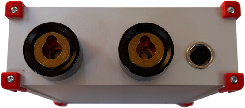
Scope of Delivery
- Sensorbox with microcontroller and connectors for Ethernet, power supply (9–12 V DC) and encoder, 12 V plug-in power supply and PoE adapter, 3-pin cable connector for voltage measurement with 5 m twisted measurement cable.
- Wire sensor (encoder) with 1.5 m cable and 5-pin cable connector.
- Gas sensor with 2 m cable and 7-pin cable connector.
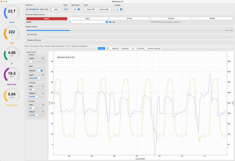
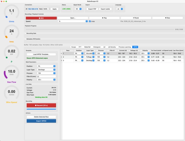
RoboScope Software for Welding Data Visualization
RoboScope is the companion PC software for the MIGAL.CO Sensorbox and is available for Windows and macOS. It serves for live visualization, analysis, recording, and diagnostics of captured welding process data – ideal for commissioning, process optimization, and troubleshooting directly at the workstation or in the laboratory.
Live Visualization (Oscilloscope)
RoboScope displays the current and voltage waveforms in real time (typically via the UDP real-time stream). This makes peaks, dips, instabilities, or unusual signal patterns immediately visible.
Spectral Analysis (FFT)
RoboScope offers a spectrum/FFT display to analyze frequency components in the measurement signals. This is particularly helpful for identifying disturbances, oscillations, or recurring patterns in the process.
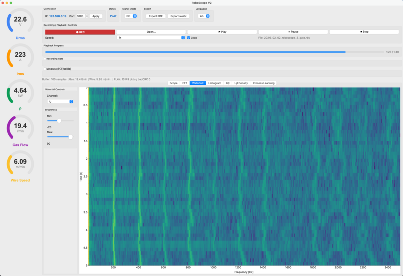
In addition to the FFT view, RoboScope provides a waterfall diagram (spectrogram). While the FFT only shows "the current moment" as a frequency spectrum, the waterfall diagram displays the frequency components over time – i.e. a 3D spectral analysis (frequency × time × amplitude/color).
- x-axis: Frequency (Hz)
- y-axis: Time (s), e.g. the last 0 to 5 seconds, with new spectra starting at the top and "scrolling" downward
- Color / Intensity: Signal strength or amplitude (typically in dB)
This allows you to see at a glance whether and when certain frequencies occur, how disturbances change, whether frequencies drift, whether there are periodic patterns, or whether oscillations only appear briefly.
This is particularly helpful for:
- Finding temporally varying disturbances (e.g. EMI pulses, load changes)
- Observing resonances/oscillations
- Making recurring patterns in the process visible
- Comparing differences between U and I over time
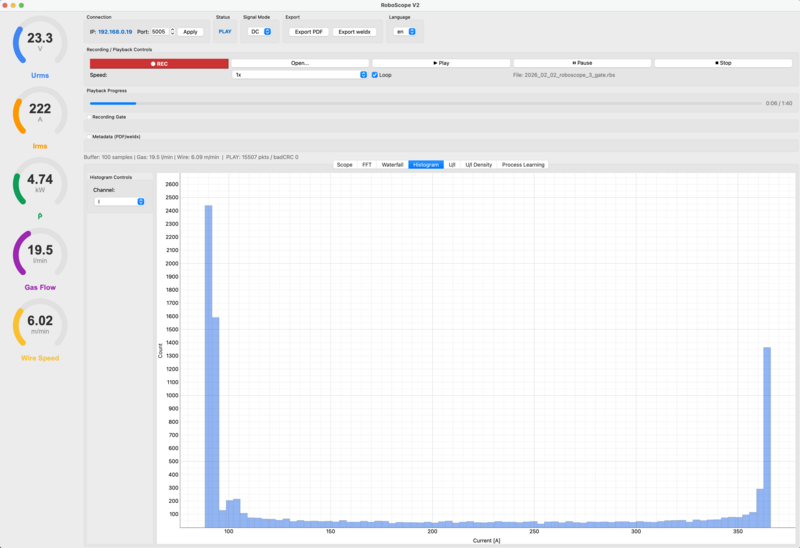
Histogram
The histogram view allows the distribution of measured values over a period to be evaluated. This quickly reveals whether the process is running stably (narrow distribution) or whether scatter and outliers occur – a valuable basis for quality assessment, job comparison, and deriving meaningful limit values.
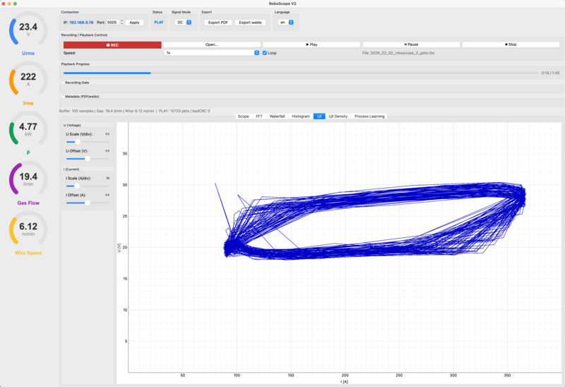
U-I Diagram (Characteristic Plot)
The U-I diagram plots voltage (U) against current (I) – i.e. not over time, but as a point cloud/curve in the characteristic space. Each measurement point from the live stream is plotted as a (U, I) pair. This provides an at-a-glance view of how the process "behaves electrically".
- Compact, stable cloud / narrow trace → Process runs smoothly, reproducibly.
- Wide cloud, outliers, jumps → Scatter, instability, unwanted events (e.g. short-circuit/arc transitions, contact problems, disturbances).
- Making process patterns visible: Many welding processes produce characteristic shapes (loops/clusters). Changes in wire feed, gas, contact tip, ground clamp, parameters, etc. shift or deform this signature – often recognizable earlier than in the time plot.
- Comparison of jobs/setups: The U-I diagram is excellent for directly comparing two jobs or two states: same shape = similar process behavior, different shape = parameter/process has changed.
- Limit values & quality logic: From the cloud, characteristic ranges can be derived (permissible "process zone"). As soon as points appear outside, RoboScope can interpret this as an indication of deviations/defects.
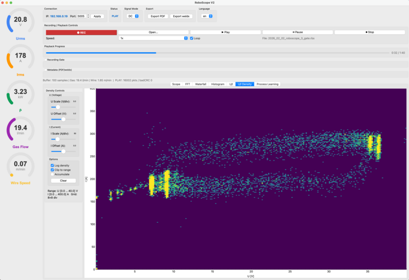
The U-I density diagram (density heatmap) shows the distribution of voltage U and current I as a point cloud with frequency coloring. Instead of displaying the signal over time, each measurement sample is placed as a point in the U-I coordinate system: x-axis = U (V), y-axis = I (A). The color intensity indicates how often a particular combination of U and I occurs – bright areas mean "frequent", dark areas mean "rare".
This allows very quick assessment of the process:
- Stability & scatter: A compact, dense cloud indicates a stable process; wide scatter indicates instability or fluctuations.
- Process states: Multiple clouds/clusters can indicate different operating states or transitions.
- Outliers: Rare events (spikes, disturbances) become visible as sparsely populated areas.
- Process window: The density distribution allows typical operating ranges to be identified and boundary areas to be defined.
Recording, Replay & Export
RoboScope can record measurement data, play it back (replay) for later analyses, and export it for external evaluations. This facilitates documentation, root cause analysis, and further processing in custom tools.
Capture welding data and export directly into a WPS-Maker 2 (.wpsx) template. Individual weld beads are recorded for a duration of 20 seconds and added to a subsequently editable list. When the list is complete, it is exported to a new .wpsx file, which can then be further edited in WPS-Maker 2.
Additionally, RoboScope supports exporting recorded measurement data in the open weldx data format.
This allows the high-resolution welding process data to be stored in a structured, long-term, and vendor-neutral manner.
The exported weldx files contain the time-resolved measurement signals (e.g. current, voltage, wire feed, gas flow) including time base and metadata, and can subsequently:
- Be supplemented with additional process and context data (e.g. weld seam geometry, component information, WPS)
- Be further processed in external analysis and research environments
- Serve as a basis for quality assurance, traceability, and AI-supported evaluation
Thus, RoboScope bridges the gap between live diagnostics at the welding station and sustainable, data-driven documentation of the welding process.
Diagnostics & Monitoring
In addition to the curves, RoboScope also provides technical insights such as timestamps, sequence numbers, and packet status. This allows quick verification of whether data arrives completely, synchronously, and plausibly – particularly helpful for network or integration questions.
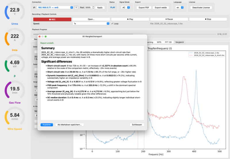
Process Comparison with AI Findings Report
Two welds. One clear report. In seconds.
The Comparison tab in RoboScope turns what normally takes hours in a welding lab into a single click: a robust, reproducible report on what has actually changed between two processes – physically, not by gut feeling.
How it works
- Load two recordings. Any .rbs files – from the lab, from pre-series testing, or straight off the Sensorbox on the shop floor. RoboScope automatically detects every individual weld inside them.
- Pick a method. Nine overlay visualizations, each highlighting a different aspect of the arc.
- Generate the AI report. One click – RoboScope extracts more than 20 physical metrics per recording, computes the relative deviations, and hands them to an AI model that turns them into a concise plain-language report.
Nine comparison methods – one click per perspective
| Method | What it shows |
|---|---|
| PSD / droplet frequency | Shifts in the dominant process frequencies – e.g. the metal-transfer rhythm |
| Short-circuit statistics | Count, rate, and duration distribution of short-circuits |
| Impedance Z(t) | Dynamic arc resistance over time |
| RMS envelope | Direct overlay of I, U, or P |
| U/I phase plot | Arc characteristic as a phase-space picture |
| Wavelet difference | Where in the time–frequency plane do the processes diverge? |
| Poincaré plot | Cycle-to-cycle stability and variability (SD1/SD2) |
| Coherence spectrum | Frequency-dependent coupling between current and voltage |
| U/I cross-correlation | Time lag between voltage and current events |
Every method ships with a short in-app explanation – understandable without a degree in signal processing.
The AI findings report
At the press of a button, RoboScope analyses either a single selected weld or every weld across both recordings and produces a structured report:
- Summary – one or two sentences describing what differs between A and B.
- Significant differences – the rated metrics with absolute values and percentage deviation. Only items whose difference is physically relevant are listed (rule of thumb: > 10 %).
The report is streamed in real time, available in German or English, can be copied or saved as a Markdown file, and is therefore ready for acceptance documentation and audits out of the box.
Which metrics feed the report
- Current & voltage: RMS, mean, standard deviation, peak-to-peak
- Power: averaged instantaneous power
- Short-circuit behavior: count, rate (Hz), mean and median duration, scatter
- Spectrum: PSD peak frequency and band power 1 – 500 Hz
- Arc impedance: mean and standard deviation of the dynamic resistance
- Stability: Poincaré metrics SD1 / SD2
- U/I coupling: mean coherence in the 50 – 500 Hz band
The comparison is built entirely on these objective metrics – the AI does not interpret data that isn't in the signal and deliberately offers no root-cause speculation and no recommendations. That keeps the report traceable and audit-friendly.
Privacy & cost control
- The Anthropic API key is stored locally and encrypted on the user's machine – not in the cloud, not in the recording.
- The analysis runs on demand: you decide when a report is generated.
Typical use cases
- WPS validation: does the production run still match the procedure qualification record?
- Machine-to-machine comparison: does robot #2 really deliver the same process as robot #1?
- Wire batch change: does the new lot have a measurable effect on the arc?
- Shift comparison: does the process drift between the morning and evening shift?
- Complaint analysis: how does the rejected bead actually differ from a known-good one?
From comparison to continuous monitoring
With the MIGAL.CO Sensorbox, a one-off comparison becomes a continuous quality tool: on request, RoboScope generates an AI model of the reference process and deploys it directly to the Sensorbox. There it monitors the welding process autonomously – no PC, no cloud – and reports anomalies via MQTT, OPC UA, Modbus TCP, or web dashboard.
From arc to decision. No detour through hours of plot-scrolling.


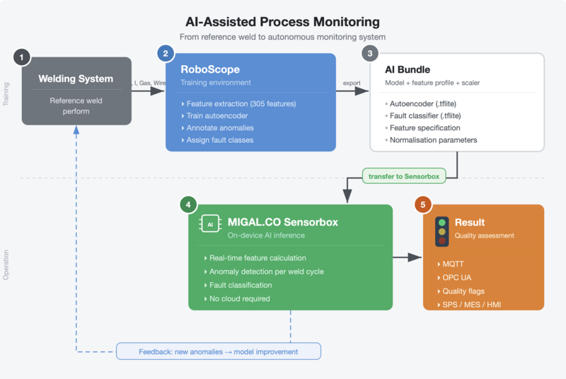
AI-Assisted Process Monitoring
The Sensorbox features an integrated AI inference engine. Trained anomaly detection models run directly on the Cortex-M7 — no PC, AI server, or cloud connection required, in real time.
This functionality is implemented on a project-specific basis, as the integration into existing production workflows — in particular the assignment of welding jobs to monitoring profiles — is individually tailored to each customer's environment.
The principle: Using the RoboScope software, a reference weld is used to create a model of the normal process state. This model is transferred to the Sensorbox, which then evaluates every welding cycle autonomously. Deviations are detected and can be forwarded to control systems via MQTT or OPC UA.
Key features:
- On-device inference with no cloud dependency
- Automatic anomaly detection based on multi-dimensional process features
- Optional fault classification (e.g. porosity, spatter, seam interruptions)
- Multiple monitoring profiles for different welding tasks
- Results as quality flags within the existing MQTT data stream
Typical project scope:
- Selection and configuration of process-relevant features
- Model training based on reference welds at the machine
- Integration with the customer's job management system (PLC, MES, or robot controller)
- Commissioning and validation in live production
Get in touch — we'll work with you to determine how AI monitoring fits into your manufacturing environment.
Additional information
 Manual4 MB
 Firmware Sensorbox 1.1.0896 KB
 RoboScope Package MacOS270 MB